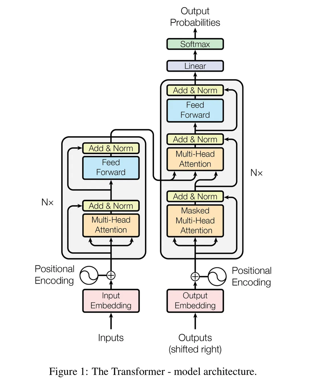
Modern language, image and video models are based on the transformer architecture proposed by researchers in 2017 in the landmark paper attention is all you need.
Before we look to the future of models like GPT-5 and SoRA we'll first need to tackle the basics. In this blog I will go over the transformer architecture piece by piece in Python and train it on the works of Shakespeare.
This article will be based on Andrej Karpathy video on transformers
What's done cannot be undone. - Macbeth
Index
- Section 1: The dataset
- Section 2: Encoding and Decoding
- Section 3: Preparing the data
- block sizes
- batch normalisation
- Section 4: The bigram model
- Embeddings
- Predictions
- Generations
- Model training
- Section 5: Self Attention
- Simple attention
- Single head attention
- Multi head attention
- Feed Forward Layer
- Section 6: Building the transformer
- The decoder block
Section 1: The Dataset
The data used to train this model can be found here
First things first, let's open up the training data and take a quick look.
inputs:
with open("./data/input.txt", 'r') as file:
    text:str = file.read()

print(f"number of characters: {len(text)}")
print(text[:300])
outputs:
number of characters: 1115394First Citizen: Before we proceed any further, hear me speak.
All: Speak, speak.
First Citizen: You are all resolved rather to die than to famish?
All: Resolved. resolved.
First Citizen: First, you know Caius Marcius is chief enemy to the people.
All: We know't, we know't.
First Citizen: Let us
Excellent! With the data loaded let's move to the next step, encoding the data.
Section 2: Encoding & Decoding
This project will use a simple character level tokenizer. This means each unique character will be represented by a numerical value. Read more about it here
We can achieve this by:
- Obtaining all the unique characters in the text
- Create a mapping of between character to index for the encoder
- Create a mapping of between index to character for the decoder
inputs:
# Get unique characters
chars = sorted(list(set(text)))

# Create a mapping from character to integer
string_to_integer = {char:i for i, char in enumerate(chars)}
# Create a mapping from integer to string
integer_to_string = {i:char for i,char in enumerate(chars)}

# Define functions to encode & decode data
encode = lambda sentence: [string_to_integer[char] for char in sentence]
decode = lambda numbers: ''.join([integer_to_string[number] for number in numbers])

# View the vocabulary list
print(f"Vocab Size: {len(chars)}")
print(f"Unique Characters: {''.join(chars)}")

# Try out some encoding and decoding
print("Encode:")
print(encode("Hey! How's it going?"))
print("Decode:")
print(decode(encode("Hey! How's it going?")))
outputs:
Vocab Size: 65

Unique Characters:
!$&',-.3:;?ABCDEFGHIJKLMNOPQRSTUVWXYZabcdefghijklmnopqrstuvwxyz

Encode:
[20, 43, 63, 2, 1, 20, 53, 61, 5, 57, 1, 47, 58, 1, 45, 53, 47, 52, 45, 12]

Decode:
Hey! How's it going?
Section 3: Preparing the data
Now that we have our simple encoder and decoder working let's tokenize the works of Shakespeare! We will:
- Encode the text
- Convert the encoded text to a PyTorch tensor
- Split the data into training and testing
- Implement batches
Let's handle the first two steps below
input:
import torch

# Tokenize the text and convert into a torch tensor
data = torch.tensor(encode(text), dtype=torch.long)

# View tensor properties
print(f"data shape: {data.shape}")
print(f"data type: {data.dtype}")
print(f"First 100 characters:\n {data[:100]}")
output:
data shape: torch.Size([1115394])

data type: torch.int64

First 100 characters:
 tensor([18, 47, 56, 57, 58,  1, 15, 47, 58, 47, 64, 43, 52, 10,  0, 14, 43, 44,
        53, 56, 43,  1, 61, 43,  1, 54, 56, 53, 41, 43, 43, 42,  1, 39, 52, 63,
         1, 44, 59, 56, 58, 46, 43, 56,  6,  1, 46, 43, 39, 56,  1, 51, 43,  1,
        57, 54, 43, 39, 49,  8,  0,  0, 13, 50, 50, 10,  0, 31, 54, 43, 39, 49,
         6,  1, 57, 54, 43, 39, 49,  8,  0,  0, 18, 47, 56, 57, 58,  1, 15, 47,
        58, 47, 64, 43, 52, 10,  0, 37, 53, 59])
Great, we've now gotten our data in a format which can be used by PyTorch. Next let's split the data into testing and validation, we can use a 90-10 split.
block size
We will now divide the training data into block sizes, there are two key reasons why we do this:
- To optimize computational efficiency : Rather than overwhelming the transformer by feeding it all the information at once, we break down the input into sequential blocks optimising processing power.
- Context: we also improve the model's comprehension of varying context lengths ranging from 1 -> block size.
In the following code snippet, we've set a block size of eight, but with an added offset of +1. This is used for predicting the next character at every position. To ensure we make eight predictions within each block, we need a block size of nine.
Let's use a smaller example demonstrating why we want five characters if we define the block size of four.
We can use the sequence of length five [10, 7, 2, 2, 15] which generates four predictions below:
| Sequence | Target |
|---|---|
| 10 -> | 7 |
| 10, 7 -> | 2 |
| 10, 7, 2 -> | 2 |
| 10, 7, 2, 2 -> | 15 |
Let's demonstrate this using a real example with our data.
input:
# Calculate the index that represents 90% of the data length
n = int(0.9 * len(data))
# First 90% of the data will be training
train_data = data[:n]
# Remaining 10 % of the data will be testing
test_data = data[n:]

# Define block size
block_size = 8
# Create a sequence of inputs for the specified block size
x = train_data[:block_size]
# Create target values for each input
y = train_data[1:block_size + 1]

# Iterate through the first block mapping input to a target
for i in range(block_size):
    context_input = x[:i + 1]
    target = y[i]
    print(f"when input is {context_input} the target is : {target}")
output:
when input is tensor([18]) the target is : 47
when input is tensor([18, 47]) the target is : 56
when input is tensor([18, 47, 56]) the target is : 57
when input is tensor([18, 47, 56, 57]) the target is : 58
when input is tensor([18, 47, 56, 57, 58]) the target is : 1
when input is tensor([18, 47, 56, 57, 58,  1]) the target is : 15
when input is tensor([18, 47, 56, 57, 58,  1, 15]) the target is : 47
when input is tensor([18, 47, 56, 57, 58,  1, 15, 47]) the target is : 58
Batching & Shuffling
To be more efficient in our computation we will organize our data blocks into batches. This approach effectively utilises the parallel computing capabilities of your GPU. This will allow us to process multiple batches at the same time, completely independently.
We will sample random locations in the data to pull out these chunks. By changing the order we process chunks we can reduce any chances of overwriting and improve the models generalisation, this process is known as shuffling.
The function get_batch() will be responsible for:
- Select Data : Select the training or validation based on user input.
- Generate Random Indices : Create a tensor with dimensions
batch_size x 1containing random indices used to shuffle the selected data. - Generate Context : Using the random indices we can generate context sequences
of dimensions
block_size x 1. - Construct Tensor : These sequences are then stacked on top of each other to create a
final tensor of
batch_size x block_sizedimensions.
Let's now do a code implementation for one training batch, so we can see how it looks!
inputs:
# Set a seed value for reproducibility
torch.manual_seed(1337)
# Maximum context length for each prediction
block_size = 8
# Number of blocks we will process in parallel
batch_size = 4


def get_batch(split: str) -> [torch.Tensor, torch.Tensor]:
    # Use training or validation data depending on user specification
    data = train_data if split == 'train' else 'val_data'
    # Generate a tensor of random indices : batch_size x 1
    ix = torch.randint(len(data) - block_size, (batch_size,))
    # Generate context sequences and stack together : batch_size x block_size
    x = torch.stack([data[i:i + block_size] for i in ix])
    y = torch.stack([data[i + 1:i + block_size + 1] for i in ix])
    return x, y


# Generate one training batch of inputs / labels
x_batch, y_batch = get_batch('train')
# View the shape and value of our inputs
print(f"inputs:\n{x_batch.shape}\n{x_batch}")
# View the shape and value of our targets
print(f"targets:\n{y_batch.shape}\n{y_batch}")

# View the context sequence and target for our batch
print("\n----------------------------------------------\n")

# Iterate through batch dimension
for batch in range(batch_size):
    print(f"\nBatch : {batch + 1}/{batch_size}")
    # Iterate through time dimension
    for t in range(block_size):
        context = x_batch[batch, :t + 1]
        target = y_batch[batch, t]
print(f"input: {context.tolist()} target: {target}")outputs:
inputs:
torch.Size([4, 8])
tensor([[24, 43, 58,  5, 57,  1, 46, 43],
        [44, 53, 56,  1, 58, 46, 39, 58],
        [52, 58,  1, 58, 46, 39, 58,  1],
        [25, 17, 27, 10,  0, 21,  1, 54]])
targets:
torch.Size([4, 8])
tensor([[43, 58,  5, 57,  1, 46, 43, 39],
        [53, 56,  1, 58, 46, 39, 58,  1],
        [58,  1, 58, 46, 39, 58,  1, 46],
        [17, 27, 10,  0, 21,  1, 54, 39]])

----------------------------------------------


Batch : 1/4
input: [24] target: 43
input: [24, 43] target: 58
input: [24, 43, 58] target: 5
input: [24, 43, 58, 5] target: 57
input: [24, 43, 58, 5, 57] target: 1
input: [24, 43, 58, 5, 57, 1] target: 46
input: [24, 43, 58, 5, 57, 1, 46] target: 43
input: [24, 43, 58, 5, 57, 1, 46, 43] target: 39

Batch : 2/4
input: [44] target: 53
input: [44, 53] target: 56
input: [44, 53, 56] target: 1
input: [44, 53, 56, 1] target: 58
input: [44, 53, 56, 1, 58] target: 46
input: [44, 53, 56, 1, 58, 46] target: 39
input: [44, 53, 56, 1, 58, 46, 39] target: 58
input: [44, 53, 56, 1, 58, 46, 39, 58] target: 1

Batch : 3/4
input: [52] target: 58
input: [52, 58] target: 1
input: [52, 58, 1] target: 58
input: [52, 58, 1, 58] target: 46
input: [52, 58, 1, 58, 46] target: 39
input: [52, 58, 1, 58, 46, 39] target: 58
input: [52, 58, 1, 58, 46, 39, 58] target: 1
input: [52, 58, 1, 58, 46, 39, 58, 1] target: 46

Batch : 4/4
input: [25] target: 17
input: [25, 17] target: 27
input: [25, 17, 27] target: 10
input: [25, 17, 27, 10] target: 0
input: [25, 17, 27, 10, 0] target: 21
input: [25, 17, 27, 10, 0, 21] target: 1
input: [25, 17, 27, 10, 0, 21, 1] target: 54
input: [25, 17, 27, 10, 0, 21, 1, 54] target: 39
Section 4: The Bigram language model
Before we build using transformer architecture let's first establish a baseline by using a very simple language model.
In short, a N-Gram model predicts the probability of the next item in a sequence based on
the previous N - 1 items. It's assumed that the probability of the next item depends
only on the previous N - 1 items, therefore
a bigram model will predict the next item based only on the previous one.
Learn more here
In practice the next word in a sentence does not depend solely on the previous one. Using this approach will allow us to draw up comparisons between this and a transformer.
Within our bigram model we will
- Define a embedding table
- Define a forward pass where we make predictions
Embeddings
Why do we need an embedding table?
We can tokenize characters, sub-words and words into a numerical representation and this is something we've already done on a character level. To demonstrate how embeddings look let's take a very simple example using word level tokenization for the following sentence :
The dog ate my homework
The dog feasted on my socks
The numeric representation of that would be
1 2 3 4 5
1 2 6 7 4 8
Here's what our data dictionary would look like:
| Word | Index |
|---|---|
| The | 1 |
| Dog | 2 |
| Ate | 3 |
| My | 4 |
| Homework | 5 |
| feasted | 6 |
| on | 7 |
| socks | 8 |
Now, The question is how could we measure closeness of each word? Or in this example how could we represent that ate and feasted have a similar meaning?
We can't use the arbitrary number we've assigned, so each word is given a unique dense vector which is learned from the data. Here is an example of if we used an embedding size of 2 x 2 for training the model.
| Word | Index | Embedding |
|---|---|---|
| The | 1 | [[0.46, 0.79], [0.20, 0.51]] |
| Dog | 2 | [[0.59, 0.05], [0.61, 0.17]] |
| Ate | 3 | [[0.07, 0.95], [0.97, 0.81]] |
| My | 4 | [[0.12, 0.50], [0.03, 0.91]] |
| Homework | 5 | [[0.26, 0.66], [0.31, 0.52]] |
| on | 7 | [[0.55, 0.18], [0.97, 0.78]] |
| socks | 8 | [[0.94, 0.89], [0.60, 0.92]] |
A visual representation:
Now, let's use a practical example where the embeddings are plotted on a two-dimensional axis. The visualisation can be found in the paper Cross-domain sentiment-aware word embeddings for review sentiment analysis
Words which share similar themes appear "closer" together within the embedding space such as light, good, sharp, best, excellent. Similarly, poor, bad are grouped close together.

In our model we will have the dimensionality of vocab_size x vocab_size. Using a high dimensional
space is usually impractical as it can increase computational complexity and dilute
meaningful relationships between words. It is common to have embedding dimensions such as 50,100, 300
however in this example our vocabulary size is 62.
Making predictions and calculating the loss
Within our forward function we will pass the inputs and target values as arguments.
- The inputs are passed into our embedding table where a prediction will be made
- The predictions will have dimensionality
batch_size x block_size x vocab_size - We will need to reshape the predictions as the loss function in PyTorch expects dimensionality
batch_size x vocab_size x block_size - We will also reshape the target values by 'flattening' them into one dimension
- Using cross entropy as our loss function we can see how well the model did at predicting
Generate
This function will generate new tokens based on the learned embeddings by
- Loop for new tokens: The function enters a loop which runs for
max_new_tokensIn each iteration the sequence will be extended by one. - Make predictions : The forward function is called and the predictions are stored in the
logitsvariable. - Isolate the last time step: The last step in the predicted values is then extracted as we want to predict what is next in the sequence based on the latest context
- Convert into probabilities : The softmax function is applied to convert predictions into probabilities.
- Select next token: Sample from the distribution to randomly select a token for each sequence based on the computed probabilities.
- Add new token to current sequence : After generating a new token it is added to the current sequence.
inputs:
import torch
import torch.nn as nn
from torch.nn import functional as F

torch.manual_seed(1337)


class BigramModel(nn.Module):

    def __init__(self, vocab_size: int):
        super().__init__()

        self.token_embedding_table = nn.Embedding(vocab_size, vocab_size)

    def forward(self, inputs, targets=None):
        # Make a prediction with our current inputs
        logits = self.token_embedding_table(inputs)  # dimensions (Batch_size, block_size, vocab_size)

        if targets is None:
            loss = None
        else:
            # Unpack each dimension
            B, T, C = logits.shape
            # Reshape logits & targets
            logits = logits.view(B * T, C)
            targets = targets.view(B * T)

            # Calculate the loss based on our predictions and the target
            loss = F.cross_entropy(logits, targets)

        return logits, loss

    def generate(self, inputs, max_new_tokens):
        # Input is (batch_size x block_size)
        for _ in range(max_new_tokens):
            # Retrieve predictions
            logits, loss = self(inputs)
            # Focus on the last time step of prediction
            logits = logits[:, -1, :]  # dimensions: (B,C)
            # Calculate probabilities by applying a softmax
            probs = F.softmax(logits, dim=-1)  # dimensions: (B,C)
            # Sample from the distribution
            inputs_next = torch.multinomial(probs, num_samples=1)  # dimensions: (B, 1)
            # Append sampled index to the running sequence
            inputs = torch.cat((inputs, inputs_next), dim=1)  # (B, T+1)
        return inputs


vocab_size = len(chars)
model = BigramModel(vocab_size=vocab_size)

logits, loss = model(x_batch, y_batch)
print(logits.shape)
print(loss)

# Let's generate 100 new characters based on an input of 0 which represents a new line
print(decode(model.generate(idx=torch.zeros((1, 1), dtype=torch.long), max_new_tokens=100)[0].tolist()))outputs:
torch.Size([32, 65])
tensor(4.8786, grad_fn=<NllLossBackward0>)

Sr?qP-QWktXoL&jLDJgOLVz'RIoDqHdhsV&vLLxatjscMpwLERSPyao.qfzs$Ys$zF-w,;eEkzxjgCKFChs!iWW.ObzDnxA Ms$3
The output is complete gibberish right now as we haven't trained our model.
Model Training
For the training of the bigram model we will use the following hyperparameters:
Optimiser: AdamLearning Rate: 0.001
To learn more about optimisers click here To learn more about learning rate click here
We will now train the model, feel free to adjust the number of steps. Once model training concludes we will generate the next 100 characters in the sequence based off a new line character.
input:
# Create torch optimizer
optimizer = torch.optim.AdamW(model.parameters(), lr=1e-3)
# Define a larger batch size
batch_size = 32

for step in range(1000):
    # Sample a batch of data
    x_batch, y_batch = get_batch('train')

    # Make a prediction and evaluate the loss
    logits, loss = model(x_batch, y_batch)
    optimizer.zero_grad(set_to_none=True)
    loss.backward()
    optimizer.step()

print(loss.item())
print(decode(model.generate(inputs=torch.zeros((1, 1), dtype=torch.long), max_new_tokens=300)[0].tolist()))output:
2.4722609519958496


Ann ied he y.
tht l acke siespre brt s RWALO:


t is
Qclide hedeist wote s ntis chendve

F blouratr; br:
Fau CAs'r to titopouthoul mar, th o avalfimingl ithaces, ms mulid t h swesed
There, lly you, to, brsqquloe h Genthil teacond sirngucerour se, urw hMar TEY3f CARDone sthiPve fallut ndr dZy, pil fa
Certainly no Shakespeare but progress is being made for a simple bigram model. Recall we are only giving the model a context of only one character.
Section 5: Self Attention
In our current implementation our tokens in the time series component do not interact with each other. To remedy this we will implement the simplest for of self attention - a summed average.
Simple attention
Let's take an example of eight tokens.
We wouldn't want the fifth token to be able to communicate with sixth, seventh and eighth as they are future tokens. The fifth token should only be able to communicate with prior tokens.
The simplest way for us to communicate with the past context is to take an average of previous elements. Granted this method is an extremely weak form of interaction as we lose a lot of information on spacial arrangements of these tokens.
We will refer to the weighted average tensor as xbow. Bag Of Words (BOW) refers to an unordered
collection of words which you can read more about here.
The xbow tensor will have the same dimensionality as our input tensor being batch size, time component, channel with
the key change being in the time component section.
To be more computationally efficient we can use matrix multiplication with this trick:
input:
# Set seed for reproducibility
torch.manual_seed(101)

# Set batch size, time component and channels
B, T, C = 4, 8, 2

# Create a Tensor of random values with dimensions B,T,C
x = torch.randn(B, T, C)

# Create a Tensor which when multiplied by our input will produce a weighted sum
# Lower traingle will tell us how much of each element will fuse
tril = torch.tril(torch.ones(T, T))

# Weights begin at Zero
weights = torch.zeros((T, T))

# Assert the future can not communicate with the past
weights = weights.masked_fill(tril == 0, float('-inf'))

# Normalize and sum
weights = F.softmax(weights, dim=1)
xbow = weights @ x
By constructing a weights matrix with dimensions Time series component x Time series component
we can simply produce a weighted average by calling weights @ x where x is the input matrix.
single head attention
When we initialise the affinities (relationships) between tokens to be zero in the line
weights = torch.zeros((T, T)) we give the weights a uniform numbers. We don't want this to be
uniform as different tokens will find other tokens more or less interesting.
For example if you are a vowel then you would look for consonants in the past context. We want to gather information from the past but do so in a data dependent way.
Self attention solves this by having every single token will emit two vectors
- A query
- A key
Query vector -> what am I looking for
Key vector -> what do I contain
The way we get the affinities between tokens is by doing a dot product between the queries and keys. A query will dot product with the keys of all the other tokens which will produce the weights.
If the key and query are aligned they will interact by a higher amount leading to a more meaningful relationship.
It is important to note that tokens do not interact across batches as they are processed independently.
Quick note:
In encoder blocks we allow the tokens to communicate with each other from the future and past
In decoder blocks we mask future context with the triangular matrix
Self attention means that the queries, keys and values all come from the same source, x
However attention is much more general such as in encoder and decoder transformers where
the queries are produced from x but the keys and values come from different sources. This is
referred to as cross-attention.
# Set seed for reproducibility
torch.manual_seed(101)
# Set batch size, time component and channels
B, T, C = 4, 8, 32
# Create a Tensor of random values with dimensions B,T,C
x = torch.randn(B, T, C)

# A single head performing self attention
head_size = 16
key = nn.Linear(in_features=C, out_features=head_size, bias=False)
query = nn.Linear(in_features=C, out_features=head_size, bias=False)
value = nn.Linear(in_features=C, out_features=head_size, bias=False)

# Forward these modules on the input tensor
k = key(x)  # Dims: B,T,head_size
q = query(x)  # Dims: B,T,head_size

# Communication
# Transpose last two dimensions for K
weights = q @ k.transpose(-2, -1) # (B,T,16) @ (B,16,T) --> (B, T, T)
# Apply scaling to control variance at initialisation
weights = weights * head_size**-0.5

tril = torch.tril(torch.ones(T,T))
# Ensure tokens do not communicate
weights = weights.masked_fill(tril==0, float('-inf'))
weights = F.softmax(weights, dim=1)

# X is private information to this token
v = value(x)
out = weights @ v
Multi-head attention
Now that we've looked at how we can create a single head of transformation, next up let's look at multi head attention.
In the code below we first define the class Head which contains the query, key, value parameters
as discussed above. There is also a forward pass where we calculate the weighted matrix of inputs.
For multi-head attention we can have multiple independent channels of communication running at once. Each head will produce its own set of attention weights and produces an output vector. These output vectors are then concatenated back together and passed through a linear projection to combine them. In the example below we also pass the combination through a dropout layer, read more about them here
class Head(nn.Module):
    """ one head of self-attention """

    def __init__(self, head_size):
        super().__init__()
        self.key = nn.Linear(n_embd, head_size, bias=False)
        self.query = nn.Linear(n_embd, head_size, bias=False)
        self.value = nn.Linear(n_embd, head_size, bias=False)
        self.register_buffer('tril', torch.tril(torch.ones(block_size, block_size)))

        self.dropout = nn.Dropout(dropout)

    def forward(self, x):
        B, T, C = x.shape
        k = self.key(x)  # (B,T,C)
        q = self.query(x)  # (B,T,C)
        # compute attention scores ("affinities")
        wei = q @ k.transpose(-2, -1) * C ** -0.5  # (B, T, C) @ (B, C, T) -> (B, T, T)
        wei = wei.masked_fill(self.tril[:T, :T] == 0, float('-inf'))  # (B, T, T)
        wei = F.softmax(wei, dim=-1)  # (B, T, T)
        wei = self.dropout(wei)
        # perform the weighted aggregation of the values
        v = self.value(x)  # (B,T,C)
        out = wei @ v  # (B, T, T) @ (B, T, C) -> (B, T, C)
        return out


class MultiHeadAttention(nn.Module):
    """ multiple heads of self-attention in parallel """

    def __init__(self, num_heads, head_size):
        super().__init__()
        self.heads = nn.ModuleList([Head(head_size) for _ in range(num_heads)])
        self.proj = nn.Linear(n_embd, n_embd)
        self.dropout = nn.Dropout(dropout)

    def forward(self, x):
        out = torch.cat([h(x) for h in self.heads], dim=-1)
        out = self.dropout(self.proj(out))
        return out
Feed Forward Layer
Feed forward neural network layers (FFNN) are positioned after each multi attention block in both the encoder and decoder parts of a transformer.
In our code the FFNN layer will consist of a
- Linear Layer
- ReLU activation function
One of the main reasons we include a FFNN layer is to introduce non-linearity to the model this allows the transformer to capture higher complexity abstractions.
class FeedFoward(nn.Module):
    """ a simple linear layer followed by a non-linearity """

    def __init__(self, n_embd):
        super().__init__()
        self.net = nn.Sequential(
            nn.Linear(n_embd, 4 * n_embd),
            nn.ReLU(),
            nn.Linear(4 * n_embd, n_embd),
            nn.Dropout(dropout),
        )

    def forward(self, x):
        return self.net(x)
Section 6: Building the Transformer
Decoder Block
We've covered all the individual parts of the Transformer so let's assemble the Decoder block. In the transformer diagram at the start of this article the decoder block is the section on the right hand side.
To improve optimisation we will also implement residual connections in the forward function of our Block class.
We've also included the Add & Normalisation layers at
self.ln1 = nn.LayerNorm(n_embd) self.ln2 = nn.LayerNorm(n_embd)
class Block(nn.Module):
""" Transformer block: communication followed by computation """

    def __init__(self, n_embd, n_head):
        # n_embd: embedding dimension, n_head: the number of heads we'd like
        super().__init__()
        head_size = n_embd // n_head
        self.sa = MultiHeadAttention(n_head, head_size)
        self.ffwd = FeedFoward(n_embd)
        self.ln1 = nn.LayerNorm(n_embd)
        self.ln2 = nn.LayerNorm(n_embd)

    def forward(self, x):
        x = x + self.sa(self.ln1(x))
        x = x + self.ffwd(self.ln2(x))
        return x
Bringing it all together
We've gone through in detail all the different concepts that go into a Transformer so let's bring it all together here:
import torch
import torch.nn as nn
from torch.nn import functional as F

# hyperparameters
batch_size = 16
block_size = 32 #
max_iters = 5000
eval_interval = 100
learning_rate = 1e-3
device = 'cuda' if torch.cuda.is_available() else 'cpu'
eval_iters = 200
n_embd = 64
n_head = 4
n_layer = 4
dropout = 0.0
# ------------

torch.manual_seed(1337)

# wget https://raw.githubusercontent.com/karpathy/char-rnn/master/data/tinyshakespeare/input.txt
with open('data/input.txt', 'r', encoding='utf-8') as f:
    text = f.read()

# here are all the unique characters that occur in this text
chars = sorted(list(set(text)))
vocab_size = len(chars)
# create a mapping from characters to integers
string_to_index = { ch:i for i,ch in enumerate(chars) }
index_to_string = { i:ch for i,ch in enumerate(chars) }
encode = lambda s: [string_to_index[c] for c in s]
decode = lambda l: ''.join([index_to_string[i] for i in l])

# Train and test splits
data = torch.tensor(encode(text), dtype=torch.long)
n = int(0.9*len(data)) # first 90% will be train, rest val
train_data = data[:n]
val_data = data[n:]

# data loading
def get_batch(split):
    # generate a small batch of data of inputs x and targets y
    data = train_data if split == 'train' else val_data
    ix = torch.randint(len(data) - block_size, (batch_size,))
    x = torch.stack([data[i:i+block_size] for i in ix])
    y = torch.stack([data[i+1:i+block_size+1] for i in ix])
    x, y = x.to(device), y.to(device)
    return x, y

@torch.no_grad()
def estimate_loss():
    out = {}
    model.eval()
    for split in ['train', 'val']:
        losses = torch.zeros(eval_iters)
        for k in range(eval_iters):
            X, Y = get_batch(split)
            logits, loss = model(X, Y)
            losses[k] = loss.item()
        out[split] = losses.mean()
    model.train()
    return out

class Head(nn.Module):
    """ one head of self-attention """

    def __init__(self, head_size):
        super().__init__()
        self.key = nn.Linear(n_embd, head_size, bias=False)
        self.query = nn.Linear(n_embd, head_size, bias=False)
        self.value = nn.Linear(n_embd, head_size, bias=False)
        self.register_buffer('tril', torch.tril(torch.ones(block_size, block_size)))

        self.dropout = nn.Dropout(dropout)

    def forward(self, x):
        B,T,C = x.shape
        k = self.key(x)   # (B,T,C)
        q = self.query(x) # (B,T,C)
        # compute attention scores ("affinities")
        wei = q @ k.transpose(-2,-1) * C**-0.5 # (B, T, C) @ (B, C, T) -> (B, T, T)
        wei = wei.masked_fill(self.tril[:T, :T] == 0, float('-inf')) # (B, T, T)
        wei = F.softmax(wei, dim=-1) # (B, T, T)
        wei = self.dropout(wei)
        # perform the weighted aggregation of the values
        v = self.value(x) # (B,T,C)
        out = wei @ v # (B, T, T) @ (B, T, C) -> (B, T, C)
        return out

class MultiHeadAttention(nn.Module):
    """ multiple heads of self-attention in parallel """

    def __init__(self, num_heads, head_size):
        super().__init__()
        self.heads = nn.ModuleList([Head(head_size) for _ in range(num_heads)])
        self.proj = nn.Linear(n_embd, n_embd)
        self.dropout = nn.Dropout(dropout)

    def forward(self, x):
        out = torch.cat([h(x) for h in self.heads], dim=-1)
        out = self.dropout(self.proj(out))
        return out

class FeedFoward(nn.Module):
    """ a simple linear layer followed by a non-linearity """

    def __init__(self, n_embd):
        super().__init__()
        self.net = nn.Sequential(
            nn.Linear(n_embd, 4 * n_embd),
            nn.ReLU(),
            nn.Linear(4 * n_embd, n_embd),
            nn.Dropout(dropout),
        )

    def forward(self, x):
        return self.net(x)

class Block(nn.Module):
    """ Transformer block: communication followed by computation """

    def __init__(self, n_embd, n_head):
        # n_embd: embedding dimension, n_head: the number of heads we'd like
        super().__init__()
        head_size = n_embd // n_head
        self.sa = MultiHeadAttention(n_head, head_size)
        self.ffwd = FeedFoward(n_embd)
        self.ln1 = nn.LayerNorm(n_embd)
        self.ln2 = nn.LayerNorm(n_embd)

    def forward(self, x):
        x = x + self.sa(self.ln1(x))
        x = x + self.ffwd(self.ln2(x))
        return x

# super simple bigram model
class BigramLanguageModel(nn.Module):

    def __init__(self):
        super().__init__()
        # each token directly reads off the logits for the next token from a lookup table
        self.token_embedding_table = nn.Embedding(vocab_size, n_embd)
        self.position_embedding_table = nn.Embedding(block_size, n_embd)
        self.blocks = nn.Sequential(*[Block(n_embd, n_head=n_head) for _ in range(n_layer)])
        self.ln_f = nn.LayerNorm(n_embd) # final layer norm
        self.lm_head = nn.Linear(n_embd, vocab_size)

    def forward(self, idx, targets=None):
        B, T = idx.shape

        # idx and targets are both (B,T) tensor of integers
        tok_emb = self.token_embedding_table(idx) # (B,T,C)
        pos_emb = self.position_embedding_table(torch.arange(T, device=device)) # (T,C)
        x = tok_emb + pos_emb # (B,T,C)
        x = self.blocks(x) # (B,T,C)
        x = self.ln_f(x) # (B,T,C)
        logits = self.lm_head(x) # (B,T,vocab_size)

        if targets is None:
            loss = None
        else:
            B, T, C = logits.shape
            logits = logits.view(B*T, C)
            targets = targets.view(B*T)
            loss = F.cross_entropy(logits, targets)

        return logits, loss

    def generate(self, idx, max_new_tokens):
        # idx is (B, T) array of indices in the current context
        for _ in range(max_new_tokens):
            # crop idx to the last block_size tokens
            idx_cond = idx[:, -block_size:]
            # get the predictions
            logits, loss = self(idx_cond)
            # focus only on the last time step
            logits = logits[:, -1, :] # becomes (B, C)
            # apply softmax to get probabilities
            probs = F.softmax(logits, dim=-1) # (B, C)
            # sample from the distribution
            idx_next = torch.multinomial(probs, num_samples=1) # (B, 1)
            # append sampled index to the running sequence
            idx = torch.cat((idx, idx_next), dim=1) # (B, T+1)
        return idx

model = BigramLanguageModel()
m = model.to(device)
# print the number of parameters in the model
print(sum(p.numel() for p in m.parameters())/1e6, 'M parameters')

# create a PyTorch optimizer
optimizer = torch.optim.AdamW(model.parameters(), lr=learning_rate)

for iter in range(max_iters):

    # every once in a while evaluate the loss on train and val sets
    if iter % eval_interval == 0 or iter == max_iters - 1:
        losses = estimate_loss()
        print(f"step {iter}: train loss {losses['train']:.4f}, val loss {losses['val']:.4f}")

    # sample a batch of data
    xb, yb = get_batch('train')

    # evaluate the loss
    logits, loss = model(xb, yb)
    optimizer.zero_grad(set_to_none=True)
    loss.backward()
    optimizer.step()

# generate from the model
context = torch.zeros((1, 1), dtype=torch.long, device=device)
print(decode(m.generate(context, max_new_tokens=2000)[0].tolist()))